← Zpět na přehled PG2 / 04 Úvod

Reprezentace

Fyzikálně založené modelování odrazivosti

Jiří Filip · ÚTIA AV ČR · ANI-PG2. PBR: parametrické modely a jejich omezení.

PDF export: 21. 10. 2026. Datum výuky není v plánu uvedeno. Šablonové datum 8. 9. 2018 není termín této přednášky.

Nativní přepis GRAFIT zachovává všech 43 stran a původní ilustrace. Výkladová upřesnění a interaktivní model jsou označeny jako doplněk.

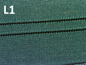
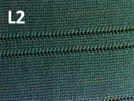
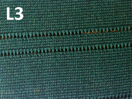
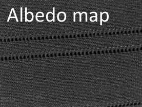
Jiří Filip · původní ilustrace · PDF strana 1
Jiří Filip · ilustrace z PDF 1

Jiří Filip · Původní PDF · strana 1

Reprezentace

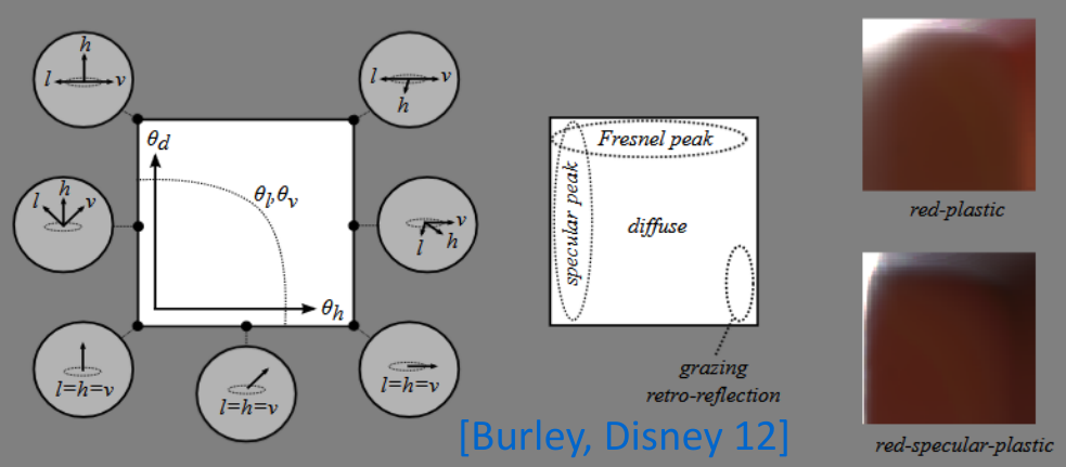
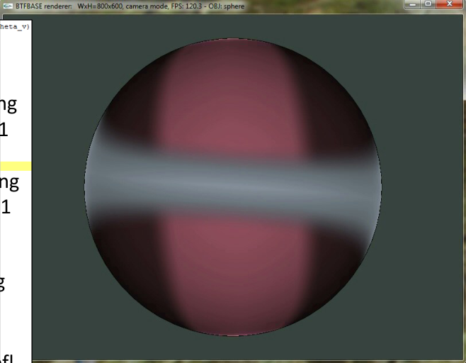
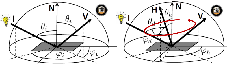
Half–difference parameterization

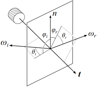
[Rusinkiewicz 1998], [Burley, Disney 2012]. Replace the incident/view pair by the half-vector and a difference direction.

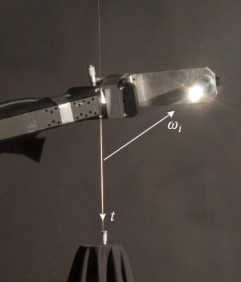
The half-vector bisects incident and outgoing directions. A local frame around it describes the remaining angular difference. The original diagrams show the convention.

Jiří Filip · původní ilustrace · PDF strana 2
Jiří Filip · ilustrace z PDF 2
Jiří Filip · původní ilustrace · PDF strana 2
Jiří Filip · ilustrace z PDF 2

Jiří Filip · Původní PDF · strana 2

Reprezentace

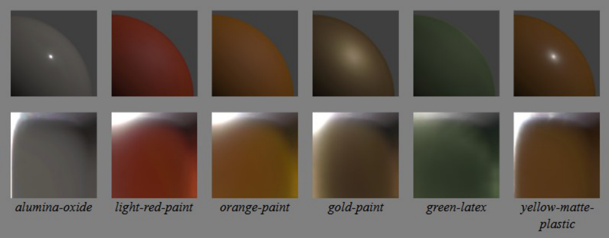
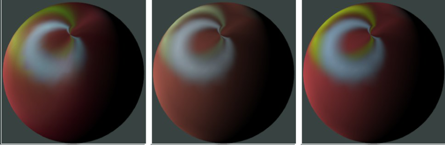
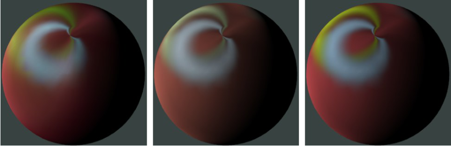
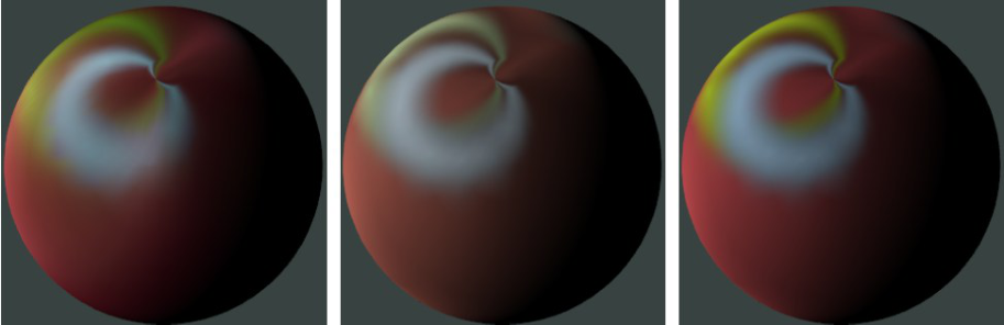
Half–difference coordinates: appearance

The original material renderings illustrate this parameterization.

A change of angular coordinates changes the representation of a BRDF, not the physical material.

Jiří Filip · původní ilustrace · PDF strana 3
Jiří Filip · ilustrace z PDF 3

Jiří Filip · Původní PDF · strana 3

Reprezentace

Compressing a BRDF

Splines [He et al. 1992], spherical harmonics [Westin et al. 1992], spherical wavelets [Schröder & Sweldens 1995], and Zernike polynomials [Koenderink et al. 1996].

A compact basis trades storage and evaluation cost against approximation error. Smooth bases can blur narrow highlights.

Jiří Filip · Původní PDF · strana 4

Reprezentace

Factorizing measured reflectance

[Kautz et al. 1999]: SVD decomposition into products of lower-dimensional functions.

[McCool et al. 2001]: homomorphic factorization with positive factors. [Suykens et al. 2003]: chained matrix factorization.

The lecture describes measured-data approximations evaluated through textures for interactive rendering.

Jiří Filip · Původní PDF · strana 5

Fotometrické stereo

Photometric stereo

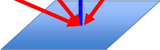
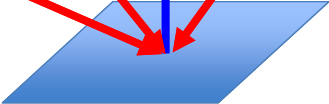
A single intensity observation cannot distinguish surface orientation from reflectance.

Keep the camera fixed and vary known illumination. Recover surface normals and albedo; integrate normals separately if a height map is required.

This differs from geometric stereo, which changes viewpoint.

Jiří Filip · původní ilustrace · PDF strana 6
Jiří Filip · ilustrace z PDF 6
Jiří Filip · původní ilustrace · PDF strana 6
Jiří Filip · ilustrace z PDF 6
Jiří Filip · původní ilustrace · PDF strana 6
Jiří Filip · ilustrace z PDF 6
Jiří Filip · původní ilustrace · PDF strana 6
Jiří Filip · ilustrace z PDF 6
Jiří Filip · původní ilustrace · PDF strana 6
Jiří Filip · ilustrace z PDF 6
Jiří Filip · původní ilustrace · PDF strana 6
Jiří Filip · ilustrace z PDF 6
Jiří Filip · původní ilustrace · PDF strana 6
Jiří Filip · ilustrace z PDF 6
Jiří Filip · původní ilustrace · PDF strana 6
Jiří Filip · ilustrace z PDF 6

Jiří Filip · Původní PDF · strana 6

Fotometrické stereo

The Lambertian observation model

For calibrated directional lights, scaled normal g = ρn converts the Lambertian model into a linear system.

Assumptions: linear camera response, known lighting, locally Lambertian reflectance, no cast shadows, saturation or interreflection in the selected observations.

Doplněk GRAFIT: alespoň tři lineárně nezávislé směry světel. Úhlové optimum je nutné vztáhnout k jasně definované normále či rovině.

Ik=ρn·lk
g=ρn

Jiří Filip · Původní PDF · strana 7

Fotometrické stereo

Calibrated photometric stereo

Stack light directions into matrix L and observed intensities into I. With three independent lights, solve for g.

The length of g yields albedo in the selected illumination convention; normalize g to obtain the surface normal.

Zero albedo gives no normal information. Near-singular lighting makes the estimate unstable.

I=Lg
g=L−1I
ρ=‖g‖,n=g/ρ

Jiří Filip · Původní PDF · strana 8

Fotometrické stereo

More than three lights

An overdetermined system uses least squares. More observations can improve robustness to random noise when the model is appropriate.

Doplněk GRAFIT: použijte QR nebo SVD místo explicitní inverze normálních rovnic. Více světel samo neodstraní systematickou chybu modelu.

g^=L+I
L+=(LTL)−1LT(rank(L)=3)

Jiří Filip · Původní PDF · strana 9

Fotometrické stereo

Robust photometric stereo

Specularities and shadows violate the simple Lambertian model.

Use robust estimation or reject inconsistent observations instead of letting a few outliers dominate the fit.

ming∑kℓ(Ik−lkTg)

Jiří Filip · Původní PDF · strana 10

Fotometrické stereo

Photometric stereo: extensions

The source compares three-light estimation with redundant least squares.

Extensions include weighted least squares, RANSAC, colour observations, near-field lights, non-Lambertian models, uncalibrated lighting and learned methods. These change the assumptions and unknowns.

Jiří Filip · Původní PDF · strana 11

Analytické modely

Analytical BRDF models

Incident direction i and outgoing direction v are parameterized by polar and azimuthal angles.

Many analytical models combine diffuse and specular terms. A Gaussian lobe is one possible approximation of a highlight.

fr(i,v)=kd/π+ksL(i,v)

Jiří Filip · Původní PDF · strana 12

Analytické modely

Reflection geometry

The original diagram contrasts diffuse reflection, specular reflection and microgeometry effects.

Masking and shadowing reduce the set of microfacets visible to both light and camera.

Jiří Filip · původní ilustrace · PDF strana 13
Jiří Filip · ilustrace z PDF 13

Jiří Filip · Původní PDF · strana 13

Analytické modely

Phong and Blinn–Phong

Phong combines ambient, diffuse and a power of the reflected-light/view alignment. Blinn–Phong uses the normal/half-vector alignment.

Doplněk GRAFIT: normalizujte směry a omezte záporné skalární součiny. Historický Phongův osvětlovací vzorec bez normalizace nelze automaticky vydávat za energeticky konzervativní BRDF.

r=2(i·n)n−i
h=(i+v)/‖i+v‖

Jiří Filip · Původní PDF · strana 14

Analytické modely

Schlick, Lafortune and Ashikhmin–Shirley

Schlick approximates the Fresnel term using reflectance at normal incidence.

Lafortune generalizes cosine lobes. Ashikhmin–Shirley includes anisotropic highlights and an energy-aware diffuse/specular combination.

Roughness shapes the distribution of microfacet normals; it is a different quantity from Fresnel reflectance.

F=F0+(1−F0)(1−cosθ)5

Jiří Filip · Původní PDF · strana 15

Analytické modely

Microfacet models

Torrance–Sparrow [1967] and Cook–Torrance [1981]: distribute small facets and combine Fresnel F, normal distribution D and geometry G.

He et al. [1991] account for wave-optical effects. The isotropy of a particular source model does not mean that every microfacet model is isotropic.

Jiří Filip · Původní PDF · strana 16

Analytické modely

Ward and anisotropic reflectance

Ward [1992] uses an exponential lobe and physically meaningful parameters; Duer [2005] discusses normalization.

The anisotropic variant controls widths along two local axes. Its normalization is model-specific; do not mix factors from different BRDF conventions.

fr=kdπ+ks1cosθicosθve−tan2θh/α24πα2
LWard=F(F0,v·h)παxαyQe−S
Q=14(i·h)2hz4
S=hx2/αx2+hy2/αy2hz2

Jiří Filip · Původní PDF · strana 17

Analytické modely

Oren–Nayar and Schlick models

Oren–Nayar describes rough diffuse reflection using Lambertian facets.

Schlick presents layered/variable-complexity approximations, including effects beyond a single smooth surface.

Jiří Filip · Původní PDF · strana 18

Analytické modely

Explicit microgeometry and threads

Westin and colleagues model microgeometry explicitly; fitting and integration can be demanding.

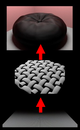
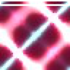
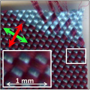
Thread-based BSDFs and woven-fabric models include the structure of yarns: [Sadeghi et al. 2013], [Xia et al. 2025].

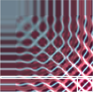
Jiří Filip · původní ilustrace · PDF strana 19
Jiří Filip · ilustrace z PDF 19
Jiří Filip · původní ilustrace · PDF strana 19
Jiří Filip · ilustrace z PDF 19
Jiří Filip · původní ilustrace · PDF strana 19
Jiří Filip · ilustrace z PDF 19
Jiří Filip · původní ilustrace · PDF strana 19
Jiří Filip · ilustrace z PDF 19

Jiří Filip · Původní PDF · strana 19

Analytické modely

Kurt et al.: anisotropic microfacets

[Kurt et al. 2010] modify the Cook–Torrance formulation for anisotropy, fitting and rendering.

The following expressions preserve the normalization displayed in this source. Symbols and factors differ from the modern GGX convention on page 22; they are not interchangeable.

fCT=kdπ+ksF(θh)D(θh)G(θi,θv)πcosθicosθv
fKurt=kdπ+ksF(v·h)D(θh,φh)4(v·h)(cosθicosθv)α

Jiří Filip · Původní PDF · strana 20

Analytické modely

Kurt et al.: repeated model comparison

The source repeats the preceding Cook–Torrance/Kurt comparison, including its two equations.

Anisotropic extension of the facet distribution; energy conservation, simple fitting and fast rendering are the properties stated by the source, not new GRAFIT performance measurements.

The repeated equations retain the source normalization and are transcribed as native formulas.

fCT=kdπ+ksF(θh)D(θh)G(θi,θv)πcosθicosθv
fKurt=kdπ+ksF(v·h)D(θh,φh)4(v·h)(cosθicosθv)α

Jiří Filip · Původní PDF · strana 21

Analytické modely

GGX: a complete specular model

h is the normalized half-vector. αx and αy are strictly positive roughness parameters along local tangent axes.

The expressions below use a consistent α notation for the source’s mixed α/σ symbols (redakční sjednocení GRAFIT). Both directions must lie above the local surface.

The separable Smith geometry term is the form shown in this lecture. Other correlated variants exist and must not be silently substituted.

fGGX=F(F0,v·h)D(h)G(i,v)4cosθicosθv
D(h)=1παxαy(hx2/αx2+hy2/αy2+hz2)2
G=1(1+Λ(i))(1+Λ(v))
Λ(v)=−1+1+(αx2vx2+αy2vy2)/vz22

Jiří Filip · Původní PDF · strana 22

Analytické modely

Disney principled reflectance

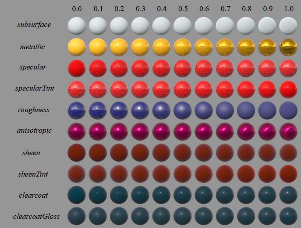
[Burley 2012]: an artist-oriented model combining diffuse reflection, a GGX/GTR2 specular lobe, GTR1 clearcoat and sheen.

Controls include base colour, metallic, roughness, specular level, anisotropy, sheen and clearcoat. They are coordinated model parameters, not independent measured physical laws.

Jiří Filip · Původní PDF · strana 23

Analytické modely

Disney: material controls

The original parameter grid illustrates how the controls change appearance.

Keep lighting and viewing conditions fixed when comparing the effect of a parameter.

Jiří Filip · původní ilustrace · PDF strana 24
Jiří Filip · ilustrace z PDF 24

Jiří Filip · Původní PDF · strana 24

Analytické modely

Fitting analytical models

Choose initial parameters, then optimize roughness, Fresnel response and anisotropy orientation. Some coefficients can be solved linearly while shape parameters require nonlinear fitting.

Loss function, sampling, initialization and local minima matter. The source mentions ALTA and MATLAB; these are source tools, not current-version recommendations.

Jiří Filip · Původní PDF · strana 25

Analytické modely

Layered BSDFs

Interfaces, scattering and absorption can be combined through multiple transport between layers.

A layered BSDF is not generally a simple sum of independent lobes. Plane-parallel approximations omit lateral transport that requires a spatial scattering model.

Jiří Filip · Původní PDF · strana 26

Anizotropie a AHL

Predicting anisotropic highlights

For an anisotropy axis U(φa), a strong response can be associated with a half-vector perpendicular to that axis.

The source uses masks around |h·U| = 0, with a finite width w (0.05 in its illustration).

Omezení zdroje: některé matematické glyfy tohoto PDF se vykreslují jako prázdná místa či černé bloky. Níže je čitelný přepis jednoznačné geometrické části; nečitelné části nejsou domýšleny.

U(φa)=(sinφa,cosφa,0)
|h·U(φa)|<w

Jiří Filip · Původní PDF · strana 27

Anizotropie a AHL

Finding multiple anisotropy axes

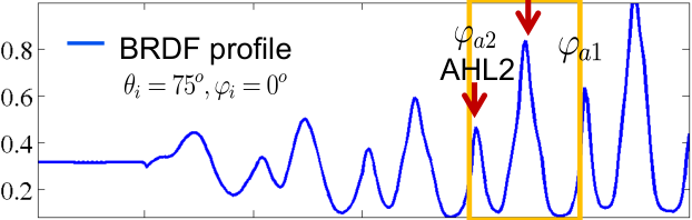
Detect prominent modes in an azimuthal profile.

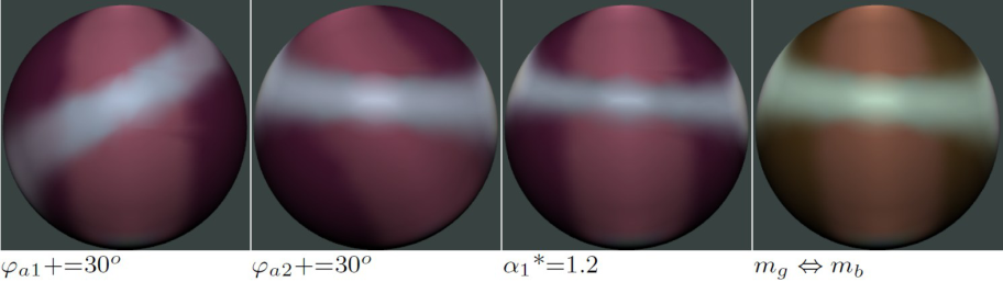
The source fits two modes independently before combining them. The original illustration shows the axes and response.

Jiří Filip · původní ilustrace · PDF strana 28
Jiří Filip · ilustrace z PDF 28
Jiří Filip · původní ilustrace · PDF strana 28
Jiří Filip · ilustrace z PDF 28
Jiří Filip · původní ilustrace · PDF strana 28
Jiří Filip · ilustrace z PDF 28
Jiří Filip · původní ilustrace · PDF strana 28
Jiří Filip · ilustrace z PDF 28

Jiří Filip · Původní PDF · strana 28

Anizotropie a AHL

Selecting informative samples

The source separates samples for anisotropy mode 1, anisotropy mode 2, specularity and shadowing.

Its illustrated configuration uses 36 samples in each of four groups: 144 samples. This is a historical setup, not a universal sampling guarantee.

Jiří Filip · původní ilustrace · PDF strana 29
Jiří Filip · ilustrace z PDF 29
Jiří Filip · původní ilustrace · PDF strana 29
Jiří Filip · ilustrace z PDF 29
Jiří Filip · původní ilustrace · PDF strana 29
Jiří Filip · ilustrace z PDF 29
Jiří Filip · původní ilustrace · PDF strana 29
Jiří Filip · ilustrace z PDF 29
Jiří Filip · původní ilustrace · PDF strana 29
Jiří Filip · ilustrace z PDF 29

Jiří Filip · Původní PDF · strana 29

Anizotropie a AHL

AHL: fitting each mode

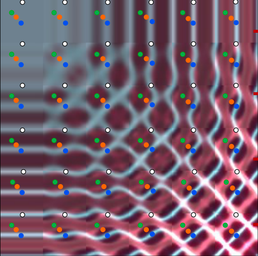
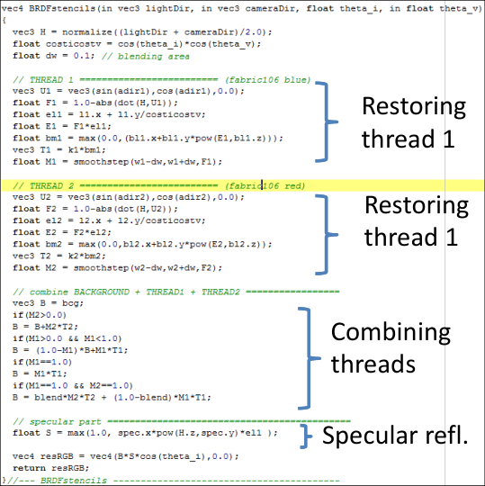
Pipeline: estimate highlight positions and anisotropy orientation; fit the elevation response; fit highlight shape and RGB response; apply thread masks.

The readable geometric position factor is F(φa) = 1 − |h·U(φa)|.

Omezení zdroje: úplný výraz výškového a intenzitního modelu je v dodaném PDF částečně nečitelný. Zachováváme slovní postup a původní PDF; nevydáváme odhad chybějících symbolů za autorovu rovnici.

F(φa)=1−|h·U(φa)|

Jiří Filip · Původní PDF · strana 30

Anizotropie a AHL

AHL: combining modes

For separated thread regions, combine the two fitted responses using their orientation masks.

The source also discusses overlapping threads, mixing, background reflectance and a specular contribution.

Omezení zdroje: úplná rovnice překryvu je částečně nečitelná. Přepsán je pouze čitelný vztah pro oddělené oblasti; podrobnosti zůstávají k ověření u autora.

Bi=Mφa1(w1)T1i+Mφa2(w2)T2i

Jiří Filip · Původní PDF · strana 31

Anizotropie a AHL

AHL: parameters and fitting

The source reports ten parameters per anisotropy mode and four global parameters. MATLAB fit/nlinfit are used in its implementation.

The reported fitting time around three seconds and roughly 144 samples belong to the author’s historical setup; GRAFIT did not remeasure them.

Source resource: stencils.zip (linked below).

Jiří Filip · Původní PDF · strana 32

Anizotropie a AHL

AHL: source comparisons

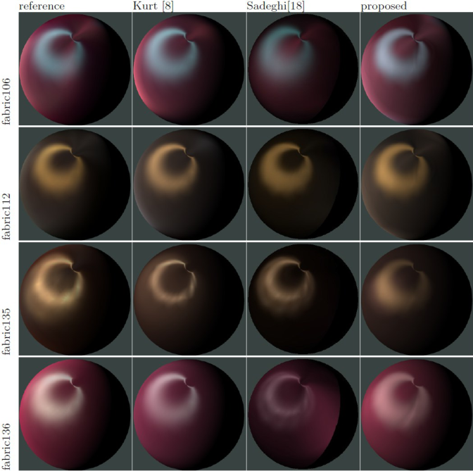
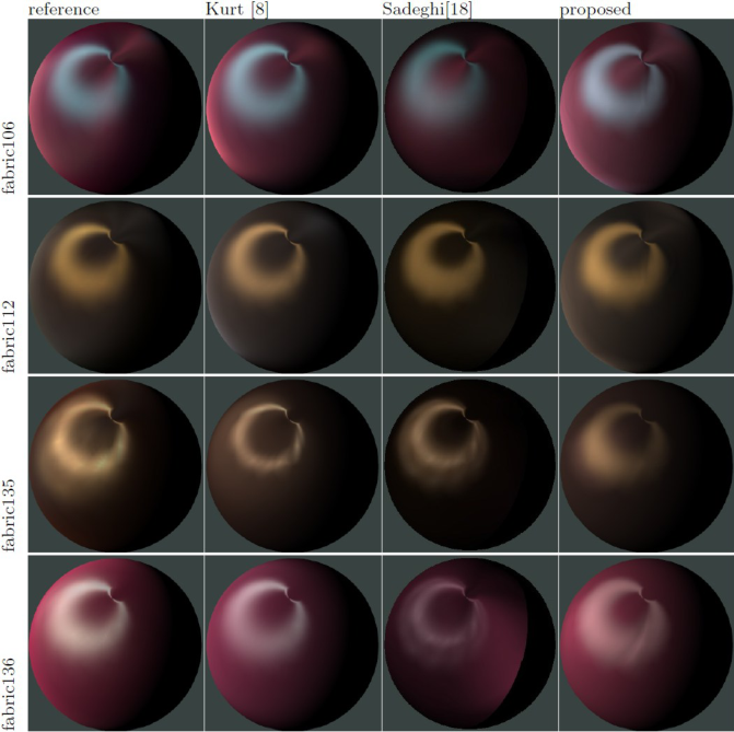
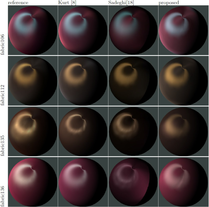
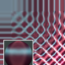
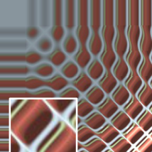
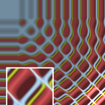
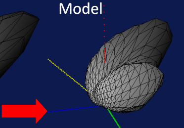
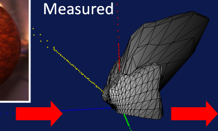
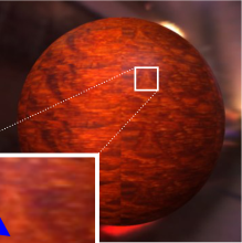
Original renderings compare the fitted model with reference appearance under point illumination.

These are author-provided results, not outputs of the interactive photometric-stereo supplement.

Jiří Filip · původní ilustrace · PDF strana 33
Jiří Filip · ilustrace z PDF 33
Jiří Filip · původní ilustrace · PDF strana 33
Jiří Filip · ilustrace z PDF 33
Jiří Filip · původní ilustrace · PDF strana 33
Jiří Filip · ilustrace z PDF 33
Jiří Filip · původní ilustrace · PDF strana 33
Jiří Filip · ilustrace z PDF 33
Jiří Filip · původní ilustrace · PDF strana 33
Jiří Filip · ilustrace z PDF 33
Jiří Filip · původní ilustrace · PDF strana 33
Jiří Filip · ilustrace z PDF 33
Jiří Filip · původní ilustrace · PDF strana 33
Jiří Filip · ilustrace z PDF 33

Jiří Filip · Původní PDF · strana 33

Anizotropie a AHL

Editing fitted appearance

Change anisotropy orientation, width and colour, or the strength of retroreflection.

Such editing changes the fitted material. It is different from recovering a unique physical microstructure.

Jiří Filip · původní ilustrace · PDF strana 34
Jiří Filip · ilustrace z PDF 34
Jiří Filip · původní ilustrace · PDF strana 34
Jiří Filip · ilustrace z PDF 34

Jiří Filip · Původní PDF · strana 34

Anizotropie a AHL

More than two anisotropy modes

The source demonstrates a material with three anisotropy modes.

Additional modes increase expressive power and also fitting complexity and the risk of ambiguity.

Jiří Filip · původní ilustrace · PDF strana 35
Jiří Filip · ilustrace z PDF 35
Jiří Filip · původní ilustrace · PDF strana 35
Jiří Filip · ilustrace z PDF 35
Jiří Filip · původní ilustrace · PDF strana 35
Jiří Filip · ilustrace z PDF 35
Jiří Filip · původní ilustrace · PDF strana 35
Jiří Filip · ilustrace z PDF 35
Jiří Filip · původní ilustrace · PDF strana 35
Jiří Filip · ilustrace z PDF 35
Jiří Filip · původní ilustrace · PDF strana 35
Jiří Filip · ilustrace z PDF 35
Jiří Filip · původní ilustrace · PDF strana 35
Jiří Filip · ilustrace z PDF 35
Jiří Filip · původní ilustrace · PDF strana 35
Jiří Filip · ilustrace z PDF 35
Jiří Filip · původní ilustrace · PDF strana 35
Jiří Filip · ilustrace z PDF 35
Jiří Filip · původní ilustrace · PDF strana 35
Jiří Filip · ilustrace z PDF 35
Jiří Filip · původní ilustrace · PDF strana 35
Jiří Filip · ilustrace z PDF 35
Jiří Filip · původní ilustrace · PDF strana 35
Jiří Filip · ilustrace z PDF 35
Jiří Filip · původní ilustrace · PDF strana 35
Jiří Filip · ilustrace z PDF 35
Jiří Filip · původní ilustrace · PDF strana 35
Jiří Filip · ilustrace z PDF 35

Jiří Filip · Původní PDF · strana 35

Anizotropie a AHL

Historical GPU demonstration

The source describes an OpenGL demonstration: about 10,000 polygons, 800 × 600 pixels and 40–70 FPS.

These numbers describe its historical hardware and implementation; they are not a performance claim for this web page.

Jiří Filip · původní ilustrace · PDF strana 36
Jiří Filip · ilustrace z PDF 36
Jiří Filip · původní ilustrace · PDF strana 36
Jiří Filip · ilustrace z PDF 36

Jiří Filip · Původní PDF · strana 36

Anizotropie a AHL

Model limitations

Balance fidelity, data size, fitting cost and rendering cost.

Parametric models may smooth sharp measured structures or miss complex effects. Original source comparisons show this limitation.

Jiří Filip · původní ilustrace · PDF strana 37
Jiří Filip · ilustrace z PDF 37
Jiří Filip · původní ilustrace · PDF strana 37
Jiří Filip · ilustrace z PDF 37
Jiří Filip · původní ilustrace · PDF strana 37
Jiří Filip · ilustrace z PDF 37
Jiří Filip · původní ilustrace · PDF strana 37
Jiří Filip · ilustrace z PDF 37

Jiří Filip · Původní PDF · strana 37

Literatura

References: representations

Source bibliography: angular representations, approximation and factorization. Full entries from the PDF follow.

BRDF representation

Rusinkiewicz, S.M., A new change of variables for efficient BRDF representation, Rendering techniques' 98, 1998, pp. 11,

Woodham, R. J. (1980). Photometric method for determining surface orientation from multiple images. Optical Engineering, 19(1), 19139

Brent Burley, Physically Based Shading at Disney, Walt Disney Animation Studios, 2012

Frankot, R. T., & Chellappa, R. (1988). A method for enforcing integrability in shape from shading algorithms. IEEE Transactions on pattern analysis and machine intelligence, 10(4), 439-451. BRDF factorization

J. Kautz and M.D. McCool. Interactive rendering with arbitrary BRDFs using separable approximations. In Proceedings of the 10th Eurographics Workshop on Rendering, pages 281-292, 1999.

M.D. McCool, J. Ang, and A. Ahmad. Homomorphic factorization of BRDFs for high-performance rendering. In E. Fiume, editor, ACM SIGGRAPH 2001, ACM Press, pages 185-194, 2001.

Jiří Filip · Původní PDF · strana 38

Literatura

References: compression and Phong

Source bibliography: compression and classical illumination models. Full entries from the PDF follow.

BRDF compression

He X. D., Heynen P. O., Phillips R. L., Torrance K. E., Salesin D. H., Greenberg D. P., A fast and accurate light reflection model, SIGGRAPH Comput. Graph. 26(2), 1992, pp. 253-254,

Westin S. H., Arvo J. R., Torrance K. E., Predicting reflectance functions from complex surfaces, SIGGRAPH '92, 1992, pp. 255-264,

Schroder P., Sweldens W., Spherical wavelets: efficiently representing functions on the sphere, SIGGRAPH '95, 1995, pp. 161-172,

Koenderink J. J., van Doorn A. J., Stavridi M., Bidirectional Reflection Distribution Function Expressed in Terms of Surface Scattering Modes, ECCV '96, 1996, pp. 28-39,

F. Suykens, K. Berge, A. Lagae, and P. Dutre, Interactive rendering with bidirectional texture functions. In Computer Graphics Forum, pages 463- 472, 2003.) BRDF models

Phong B.T., Illumination for Computer Generated Images, Communications of the ACM, 18(6), pp. 31-317, 1975,
Jiří Filip · Původní PDF · strana 39

Literatura

References: analytical reflectance

Source bibliography: analytical BRDF models. Full entries from the PDF follow.

BRDF models (continued)

Blinn J.F., Models of Light Reflection for Computer Synthesized Pictures, Computer Graphics Proceedings, pp.192-198, 1977,

Neumann L., Neumann A., Szirmay-Kalos L., Compact metallic reflectance models, Computer Graphics Forum, 18(13), 1999,

Ashikhmin M., Shirley, P., An Anisotropic Phong Light Reflection Model, Journal of Graphics Tools, 5(2), pp. 25-32, 2000,

Torrance K. and Sparrow E., Theory for Off-Specular Reflection from Rough Surfaces, Journal of the Optical Society of America, 57(9), pp. 1105-1114, 1967,

Cook R. L., Torrance K. E., A reflectance model for computer graphics, ACM SIGGRAPH 1981, 15(3), pp. 307-316, 1981,

He X., Torrance K. E.m, Sillion F.X., Greenberg D.P., A Comprehensive Physical Model for Light Reflection, Computer Graphics, 25(4), 1991,

Jiří Filip · Původní PDF · strana 40

Literatura

References: repeated source page

This page repeats the preceding bibliography page in the source PDF. It is retained in the page map for complete source coverage.

BRDF models (continued)

Blinn J.F., Models of Light Reflection for Computer Synthesized Pictures, Computer Graphics Proceedings, pp.192-198, 1977,

Neumann L., Neumann A., Szirmay-Kalos L., Compact metallic reflectance models, Computer Graphics Forum, 18(13), 1999,

Ashikhmin M., Shirley, P., An Anisotropic Phong Light Reflection Model, Journal of Graphics Tools, 5(2), pp. 25-32, 2000,

Torrance K. and Sparrow E., Theory for Off-Specular Reflection from Rough Surfaces, Journal of the Optical Society of America, 57(9), pp. 1105-1114, 1967,

Cook R. L., Torrance K. E., A reflectance model for computer graphics, ACM SIGGRAPH 1981, 15(3), pp. 307-316, 1981,

He X., Torrance K. E.m, Sillion F.X., Greenberg D.P., A Comprehensive Physical Model for Light Reflection, Computer Graphics, 25(4), 1991,

Jiří Filip · Původní PDF · strana 41

Literatura

References: rough diffuse and microfacet models

Source bibliography: Oren–Nayar, Schlick, Lafortune, fabric, GGX and surveys. Years and names are reproduced as listed; they are not silently “corrected” by this adaptation.

BRDF models (continued)

Nayar S. K., Oren M., Generalization of the Lambertian Model and Implications for Machine Vision, International Journal of Computer Vision, 14(-), pp. 227-251, 1995,
Schlick, C., An Inexpensive BRDF Model for Physically-based Rendering, Computer Graphics Forum, 13(3), pp. 149-162, 1994,
Lafortune E. P., Foo S. Ch., Torrance K. E., Greenberg, D. P., Non-Linear Approximation of Reflectance Functions, Computer Graphics, 31, pp. 117- 126, 1997,

Sadeghi, Iman, et al. A practical microcylinder appearance model for cloth rendering. ACM Transactions on Graphics (TOG) 32.2 (2013): 1-12,

Walter, Bruce, et al. Microfacet models for refraction through rough surfaces. Rendering techniques 2007 (2007): 18th,

Guarnera, Darya, et al. BRDF representation and acquisition. Computer graphics forum. Vol. 35. No. 2. 2016,

Kavoosighafi, Behnaz, et al. Deep SVBRDF acquisition and modelling: A survey. Computer Graphics Forum. Vol. 43. No. 6. 2024.

Jiří Filip · Původní PDF · strana 42

Literatura

References: layers and threads

Source bibliography: layered appearance [Jakob et al. 2014] and thread structure [Xia et al. 2025]. Full entries from the PDF follow.

BRDF models (continued)

Jakob, W., d'Eon, E., Jakob, O., & Marschner, S. (2014). A comprehensive framework for rendering layered materials. ACM Transactions on Graphics (ToG), 33(4), 1-14.

Xia, M., Zhang, Z., Chaturvedi, S., Yi, Y., Wu, R., Rushmeier, H., & Dorsey, J. (2025). Predicting fabric appearance through thread scattering and inversion. ACM Transactions on Graphics (TOG), 44(4), 1-12.

Jiří Filip · Původní PDF · strana 43

Obsah přednášky

Poznámky

Textový výklad této strany

Kalibrované fotometrické stereo · GRAFIT

xz

Výpočetní doplněk GRAFIT: syntetické intenzity, nikoli naměřená data. Tři jednotková světla mají azimut 0°,120°,240° a polární úhel 35° od z. Normála se odklání nejvýše o35°, takže bez přidané odchylky nejsou stíny. I=ρ(n·l); konstanty osvětlení včetně Lambertova faktoru jsou absorbovány do kalibrace. Odchylka se přičítá jen první intenzitě, záporný výsledek se ořízne na0. Přesně tři rovnice nemají redundanci pro detekci chyby. Zelená: skutečná normála; oranžová: odhad; graf zobrazuje pouze projekci xz.